-
RCA: sparsity-based dimension reduction and super-resolution algorithm.
Python source code available here: rca.tar.gz
The method
RCA (Resolved Components Analysis, [1]) aims at characterizing globally a space-variant PSFs field. Given a set of aliased and noisy images of unresolved objects (stars images from a telescope for instance), RCA estimates well-resolved and noise-free PSFs at the observations positions, in particular, exploiting the spatial correlation of the PSFs across the imaging system field of view (FOV). Let consider a set of p images of unresolved objects $$\mathbf{y}_1,\dots,\mathbf{y}_p$$ in a given instrument FOV and $$\mathbf{x}_1,\dots,\mathbf{x}_p$$ the corresponding ideal PSFs; these images are treated as column vectors and we note $$\mathbf{Y} = [\mathbf{y}_1,\dots,\mathbf{y}_p]$$ and $$\mathbf{X} = [\mathbf{x}_1,\dots,\mathbf{x}_p]$$. RCA minimizes $$ \frac{1}{2}{\|\mathbf{Y}-\mathcal{F}(\mathbf{X})\|_F^2}$$, where $$\mathcal{F}$$ accounts for the observed stars downsampling; this is done subject to several constraints over $$\mathbf{X}$$:
- Positivity constraint: each PSF $$\mathbf{x}_j$$ should be positive;
- Low rank constraint: each estimated PSF is forced to be a linear combination of a few number esimated of "eigen" PSFs; $$\mathbf{x}_j = \sum_{i=1}^r a_{ij} \mathbf{s}_i$$, with $$r \ll p$$ or equivalently, $$\mathbf{X} = \mathbf{S}\mathbf{A}$$, $$\mathbf{S}$$ and $$\mathbf{A}$$ being low rank matrices;
- Piece-wise smoothness constraint: we can assume that the vectors $$\mathbf{x}_j$$ are structured; promoting the sparsity of the "eigen" PSFs $$\mathbf{s}_j$$ in an appropriate dictionary $$\boldsymbol{\Phi}$$ allows to capture the spatial correlations within the PSFs themselves;
- Proximity constraints: the more two PSFs are close in the FOV, the more they should be similar; the p values relative to the $$i^{th}$$ line of $$\mathbf{A}$$ correspond to the contribution of the $$i^{th}$$ "eigen" PSF across the field of view; therefore the PSFs field regularity is enforced by constraining $$\mathbf{A}$$'s lines; specifically, each line is calculated as a sparse linear combination of spatial frequencies atoms: $$\mathbf{A} = \boldsymbol{\alpha}\mathbf{U}^T$$ (see Fig.1).
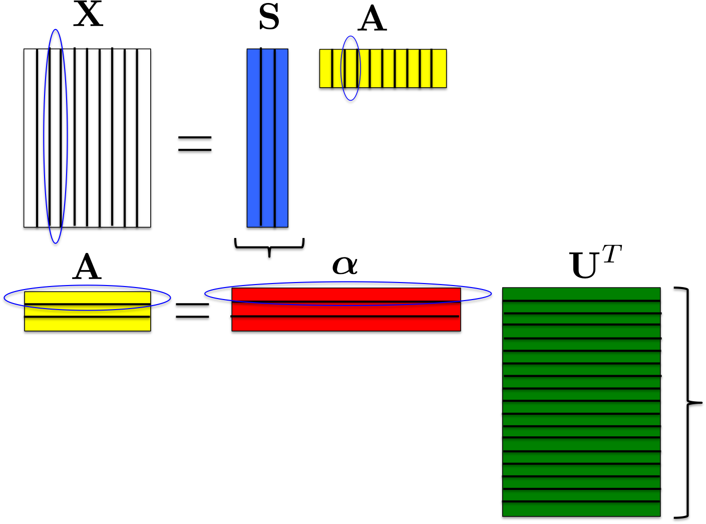
Figure 1: Data matrix factorization. $$\mathbf{U}$$ columns correspond to different spatial frequencies of the PSFs field. Hence RCA solves the following problem:
\[ \underset{\boldsymbol{\alpha},\mathbf{S}}\min \frac{1}{2}{\|\mathbf{Y}-\mathcal{F}(\mathbf{S}\mathbf{A})\|_F^2} + \sum_{i=1}^r \|\mathbf{w}_i\odot\boldsymbol{\Phi}\odot\mathbf{s}_i\|_1\; \text{s.t.}\; \|\boldsymbol{\alpha}[l,:]\|_0 \leq \eta_l, \; l=1....r \;\text{and } \mathbf{S}\boldsymbol{\alpha}\mathbf{U}^T \geq 0. \]The operator $$\mathcal{F}$$ is set according to the resolution enhancement factor specified. Besides, this operator also accounts for the observed images subpixel offsets which are automatically estimated. $$\boldsymbol{\Phi}$$ is a user-chosen redundant dictionary. The frequency dictionary $$\mathbf{U}$$ is automatically built based on the observations $$\mathbf{y}_i$$ locations in the imaging instrument FOV. The sparsity parameters $$(\mathbf{w}_i)_i$$ and $$(\eta_l)_l$$ as well are automatically selected. The number of "eigen" PSFs, r, has to be specified. It might be automatically reduced depending of the signal-to-noise ratio, the observations resolution and the sample size. A principal components analysis should provide the user a good first guess for r.
Numerical examples
RCA was tested on set on 500 Euclid telescope simulated PSFs. The simulated observables were downsampled to Euclid telescope resolution and corrupted with a white gaussian noise. Four examples of recovered PSFs are given in Fig.2. In this example, 10 "eigen" PSFs were required. We compare the result to the PSFs obtained from the software PSFEx, using the same observations.
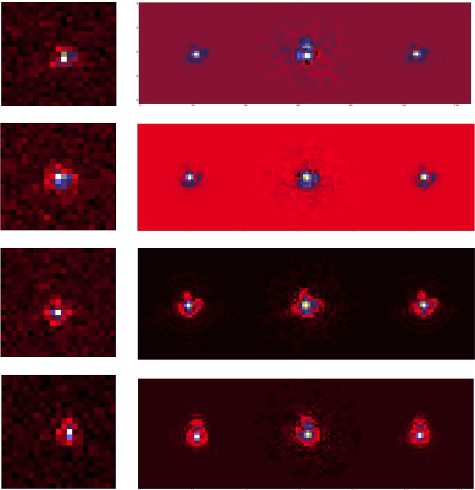
Figure 2: Euclid PSFs restoration. From the left to the right: observed PSFs, original PSFs, PSFEx restored PSFs, RCA restored PSFs. As it can be seen from these reconstructions, RCA handles the undersampling and the PSFs spatial variability, with both noise-robustness and a high visual quality.
Article
-
- [1] F. M. Ngolè Mboula, J.-L. Starck, K. Okomura, J. Amiaux, P. Hudelot. Constraint matrix factorization for space variant PSFs field restoration, Inverse Problems. Available here.