One fundamental problem in signal processing involves decomposing an image or signal into superposed contributions from different sources. Morphological Component Analysis (Starck et al. 2004) addresses this class of problems using sparsity as a tool to differentiate several contributions in a signal, each one having a specific morphology.
[metaslider id=1863]
See more illustrations on the MCA Experiments page.
The MCA Framework
Formally, the observed signal $$y$$ is modelled as a noisy linear mixture of distinct morphological components $$\left(x_k \right)_{k=1,\cdots,K}$$:
\[ y = \sum_{k=1}^K x_k + \epsilon = \sum_{k=1}^K \Phi_k \alpha_k + \epsilon ~ , ~ \epsilon \sim \mathcal{N}(0,\sigma_\epsilon^2)\]
MCA assumes that a dictionary can be built by amalgamating several sub-dictionaries $$\left(\Phi_1,\cdots,\Phi_K\right)$$ such that, for each $$k$$, the representation of $$x_k$$ in $$\Phi_k$$ is sparse and not, or at least not as sparse, in other $$\Phi_l, l \ne k$$. In other words, the sub-dictionaries $$\left(\Phi_k\right)_k$$ must be mutually incoherent. Thus, the dictionary $$\Phi_k$$ plays a role of a discriminant between content types, preferring the component $$x_k$$ over the other parts.
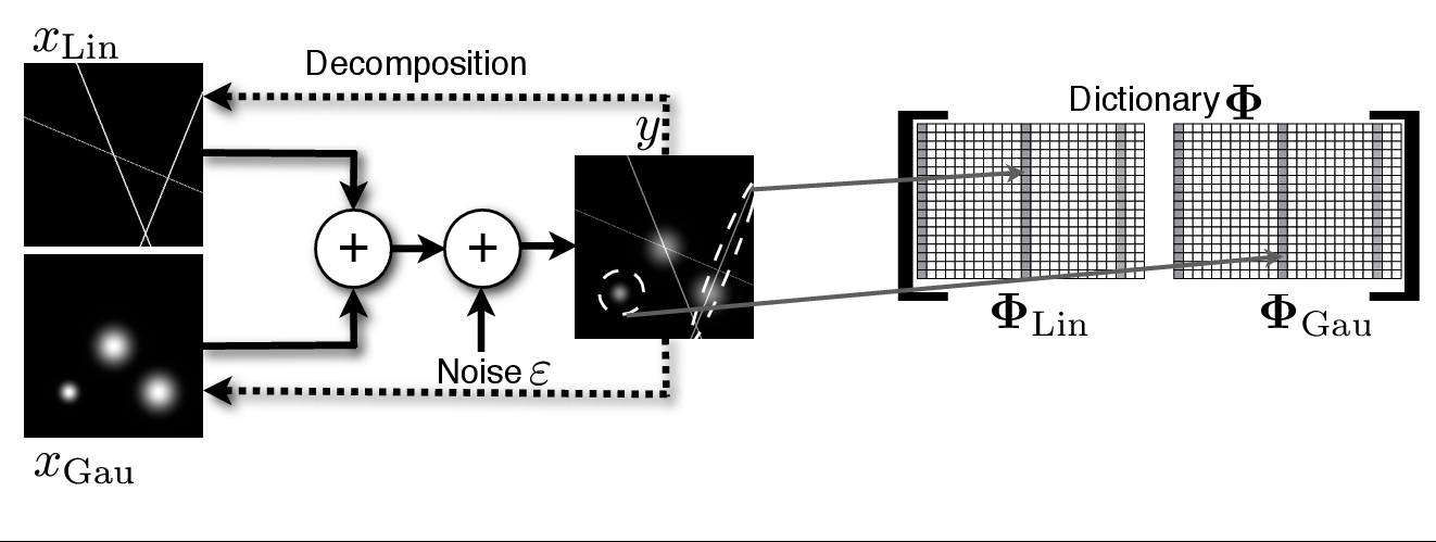
Figure 1 gives an illustrative example. Let our image contain lines and Gaussians. Then the ridgelet transform (here $$ \Phi_{Lin}$$) would be very effective at sparsely representing the global lines and poor for Gaussians. On the other hand, wavelets (here $$ \Phi_{Gau}$$) would be very good at sparsifying the Gaussians and clearly worse than ridgelets for lines.
To effectively solve the separation problem, Starck et al. (2004b) and Starck et al. (2005a) proposed the MCA algorithm which estimates each component $$\left(x_k \right)_{k=1,\cdots,K}$$ by solving the following optimization problem:
\[ \min_{\alpha_1,\cdots,\alpha_K} ~ \sum_{k=1}^K \parallel \alpha_k \parallel ^p_{p} ~ \text{st.} \parallel y – \sum_{k=1}^K \Phi_k \alpha_k \parallel_2 \leq \sigma ~,\]
where $$\parallel \alpha \parallel^p_p$$ is sparsity-promoting (the most interesting regime is for $$0 \leq p \leq 1$$), and $$\sigma$$ is typically chosen as a constant times $$\sqrt{N}\sigma_\epsilon$$.
Applications
 Supernovae Detection: Artifact removal for supernovae detection in the SuperNova Legacy Survey (Moller et al. (2015))
Publications
- J.L. Starck, F. Murtagh, and J. Fadili, Sparse Image and Signal Processing: Wavelets, Curvelets, Morphological Diversity , Cambridge University Press, Cambridge (GB), 2010. (ISBN-10: 0521119138; 336-pp. monograph).
- M. Elad, J.-L Starck, D. Donoho and P. Querre, “Simultaneous Cartoon and Texture Image Inpainting using Morphological Component Analysis (MCA)”, Journal on Applied and Computational Harmonic Analysis ACHA , Vol. 19, pp. 340-358, November 2005.
- J.-L. Starck, M. Elad, and D.L. Donoho, “Image Decomposition Via the Combination of Sparse Representation and a Variational Approach”, IEEE Transaction on Image Processing , 14, 10, pp 1570–1582, 2005 .
- J.-L. Starck, M. Elad, and D.L. Donoho, “Redundant Multiscale Transforms and their Application for Morphological Component Analysis”, Advances in Imaging and Electron Physics , 132, 2004.